User Interfaces and Visualization

This document corresponds to the Annotation and Visualization example folder within a VIAME desktop installation. Contained in this example are launch scripts for some of the more common graphical user interfaces (GUIs) within VIAME, alongside CLI scripts for visualizing or extracting data from either computed or manually annotated detection files. Examples of the latter include drawing detection boxes on images, extracting image chips around detections, or extracting images from video files at frame rates indicated within the metadata of truth files.

DIVE Interface

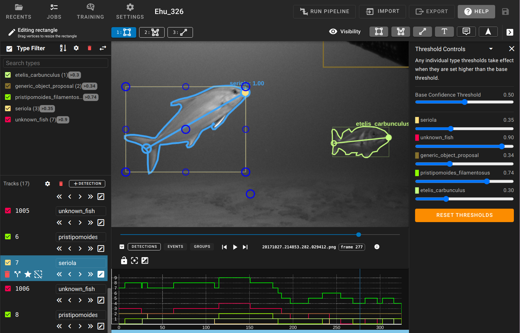
The DIVE interface is the most generically useful GUI within VIAME, and is the recommended default interface to use for many problems. The biggest allure is its ability to annotate multiple image sequences or videos, train AI models across these multiple sequences, then run the trained models on new sequences. This process can then be repeated with the help of the newly trained models to potentially annotate data faster, then train a newer model on significantly more data. Additional information about how to use the DIVE interface can be found in its dedicated user manual and additionally in the tutorial videos. The interface can be launched via double clicking the “launch_dive_interface” script, either in this directory or at the top level of the installation. Alternatively a smaller version of DIVE can be installed independently of VIAME, which contains no algorithms or AI-assisted annotation.

Interactive Segmentation in DIVE

DIVE provides interactive segmentation, allowing users to click on objects (foreground and background points) to generate segmentation masks in real time. The segmentation service is started automatically by DIVE based on the configured segmenter in the DIVE settings. Several segmentation backends are available:

Watershed (default)

Uses OpenCV’s watershed algorithm for point-based segmentation. Users provide foreground points (marking the object) and background points (marking areas to exclude). This is the lightest-weight option and does not require a GPU or any add-ons. Works best for objects with clear color boundaries.

SAM2 (SAM2 add-on)

Uses Meta’s SAM2 (Segment Anything Model 2) for point-based segmentation. Provides significantly better segmentation quality than watershed, especially for complex object boundaries. Requires less system resources than SAM3 but lacks the ability to perform text queries. Requires a GPU and the SAM2 add-on.

SAM3 (SAM3 add-on)

Uses SAM3 for both point-based and text-based segmentation. In addition to click-based segmentation, users can type a text description of the object to segment (e.g., “fish”, “scallop”). Requires a GPU and the SAM3 add-on. This is the most capable interactive segmentation option.

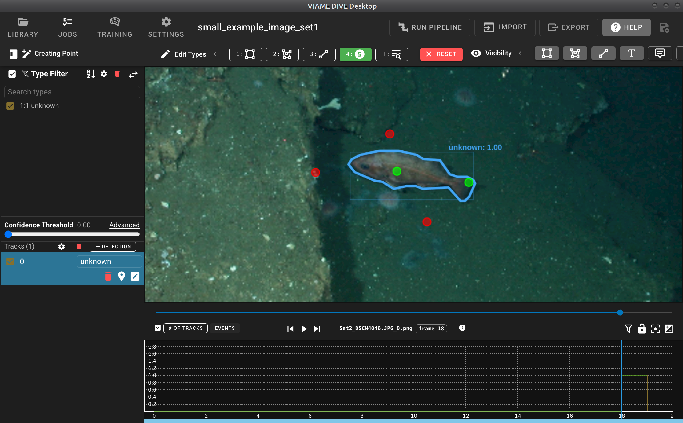
Point-based interactive segmentation in DIVE. The user clicks foreground (green) and background (red) points to generate a segmentation mask around the object.

Text queries can also be run as batch pipelines to detect, segment, and track objects across entire image sets or videos. See the SAM3 Text-Prompted Detection and Tracking section in the search and rapid model generation examples for details.

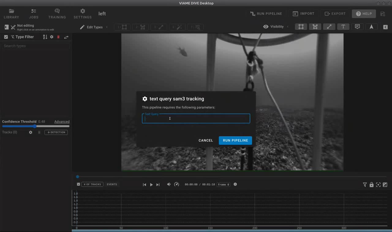
SAM3 text query dialog in DIVE. Users enter a text description of the object to detect and track across the video.

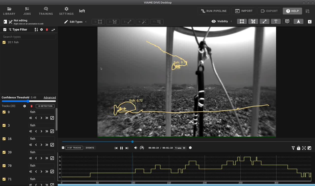
Results of a SAM3 text query showing automatically detected and tracked fish with segmentation outlines.

To manually start the interactive segmentation service outside of DIVE (e.g., for scripting or integration with other tools):

source /path/to/VIAME/install/setup_viame.sh
python -m viame.core.interactive_segmentation \
  --config configs/pipelines/interactive_segmenter_watershed.conf

VIEW Interface

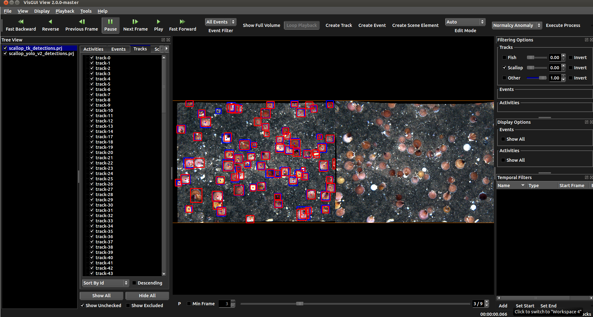
As part of the VIVIA package, the VIEW annotation interface is useful for displaying detections, their respective probabilities, for running existing automated detectors, and for making new annotations in imagery or video. Its main weakness is that it can only load a single sequence at a given time. Its strengths are that it has a number of enhancements for annotating very large images, e.g. satellite imagery in the form of geotiffs or nitfs. Some people also prefer its annotation style. Training over multiple sequences can be performed with the help of project folders

VIEW can either be pointed directly to imagery, pointed to a compressed video file (see [install-dir]/configs/prj-*/for_videos), or given an input .prj file that points to the location of input imagery and any optional settings (e.g. groundtruth, computed detections, and/or homographies for the input data). If you just want to use the tool to make annotations you don’t need to specify the later three, and just need to set a DataSetSpecifier or [reccommended] use the File->New Project option to load imagery directly without a prj file. Also, see the below example guide and videos. The VIEW interface can be launched via the “launch_view_interface” script.

Manual Annotation Guide (PDF)

Example Video Overviews (Youtube)

Notable VIEW Shortcut Keys

• r = Zoom back to the full image

• hold ctrl + drag = create a box in annotation mode (create detection/track)

VIEW Project File Overview

Examples of the optional contents of loadable prj files are listed below for quick reference. For those not familiar with the tool, downloading the above manual is best. Project files are no longer required to be used (imagery can be opened directly via the ‘New Project’ dropdown), however, these are listed here for advanced users who may want to configure with multiple homographies.

Note: The list is not complete, but currently focusing on the most used (and new) parameters

• DataSetSpecifier = filename(or glob) Filename with list of images for each frame or glob for sequence of images

• TracksFile = filename Filename containing the tracks data.

• TrackColorOverride = r g b rgb color, specified from 0 to 1, overrides the default vpView track color for this project only

• ColorMultiplier = x Event and track colors are scaled by the indicated value. Can be used in conjunction with the TrackColorOverride

• EventsFile = filename Filename containing the events data.

• ActivitiesFile = filename Filename containing the activity data.

• SceneElementsFile= filename Filename containing the scene elements (in json file).

• AnalysisDimensions = W H Dimension (in pixel/image coordinates) of AOI. Ignored when using a mode that leverages image corner points for imagetransformation.

• OverviewOrigin = U V Offset of image data such that “0, 0” occurs at the AOI origin. Should always be negative #’s. Like AnalysisDimensions, unused when image corner points are used.

• AOIUpperLeftLatLon = lat lon Required for “Translate image” mode of corner point usage (Tools->Configure->Display); also required for displaying an AOI when the source imagery isn’t ortho-stabilized

• AOIUpperRightLatLon = lat lon

• AOILowerLeftLatLon = lat lon

• AOILowerRightLatLon = lat lon If the UpperLeft and LowerRight are specified, an AOI “box” can be displayed. Depending on the nature of the homography controlling image display / transformation, additional corner point may improve the designation of the region.

• FrameNumberOffset = N Positive value to offset imagery relative to the track/event data. A value of 3 would mean that the 1st image would correspond to track frame 2 (0-based numbering)

• ImageTimeMapFile = filename Specifies file containing map of “filename <space> timestamp (in seconds)” one line per frame. The file can be created via File->Export Image Time Stamps

• HomographyIndexFile = filename Specifies file containing frame number/timestamp/homography sequence for all frames specified by the DataSetSpecifier. If the tag is set and the number of homographies match the image source count, the “Image-loc“‘s of the tracks (not the “Img-bbox”) are stored in coordinate frame mapped to by the homographies. This enables track trails during playback (for source imagery that isn’t stored in stabilized form)

• HomographyReferenceFrame = frame index Specifies the frame to use as the reference homography frame for stabilizing the video (if homographies are present). If, instead of stabilizing the video, the homographies should be used to stabilize the tracks, set the HomographyReferenceFrame to -1 (defaults to 0).

• FiltersFile = filename (note, support not yet in master) Specifies file containing definitions of spatial filters for the project. The coordinate system (lat/lon or image/pixels) must be consistent between states when the filters are saved versus when the project / filter file is loaded.

• IgnoreImageCoords = true/false (note, support not yet in master) In the world mode, ignores the image bounding box data and shows a head (point/dot) at the end of the track tail. This parameter only affects the track head and not the tail.

• ColorWindow = W (defaults to 255) Window / range of input color values that will be mapped. The value gives the total range, not the distance from the median.

• ColorLevel = L (defaults to 127) Input color value that will be mapped to the median output value, and also serves as the median value of the input color range.

SEARCH Interface

The search interface is a dedicated interface for performing image search for a particular exemplar image, be it a specific species or an object with a particular attribute or characteristic. A secondary proceedure allows adjudacating the system-generated responses for this query and the generation of a model for a new object category. This proceedure has a few trade offs compared to traditional approaches, including the ability to rapidly generate a machine learning model faster, at the risk of decreased accuracy (depending on the problem).

For additional information, see the dedicated example for it.

CLI Tools

Standalone utility scripts in this folder include the following. Each of these is designed to take in a folder of videos, folder of images, or a folder of folders of images, see default input folder structure.

• draw_detections_on_frames - Draw detections stored in some detection file onto frames

• extract_chips_from_detections - Extract image chips around detections or truth boxes

• extract_frames - Extract all frames in videos in the input folder

• extract_frames_with_dets_only - Extract frames with detections only in the input

Simple Pipeline UIs

Lastly, there are additionally simpler GUIs which can be enabled in .pipe files.

For directly running and editing pipeline files, see the KWIVER documentation.

One example of this is the ‘simple_display_pipeline’. This script launches a pipeline containing an OpenCV-based display window, which prints out detections as they are being processed by the pipeline.