Object Detection Examples
Detection Overview
This document corresponds to this example online, in addition to the object_detection example folder in a VIAME installation.
This folder contains assorted examples of object detection pipelines running different detectors such as YOLOv2, ScallopTK, Faster RCNN, and others. Several different models are found in the examples, trained on a variety of different sensors. It can be useful to try out different models to see what works best for your problem.
Running the Command Line Examples
Each run script contains 2 calls. A first (‘source setup_viame.sh’) which runs a script configuring all paths required to run VIAME calls, and a second to ‘kwiver runner’ running the desired detection pipeline. For more information about pipeline configuration, see the pipeline examples. Each example processes a list of images and produces detections in various format as output, as configured in the pipeline files.
Each pipeline contains 2-10 nodes, including a imagery source, in this case an image list loader, the actual detector, detection filters, and detection writers. In the habcam example an additional split processes is added early in the pipeline, as habcam imagery has stereo pairs typically encoded in the same png.
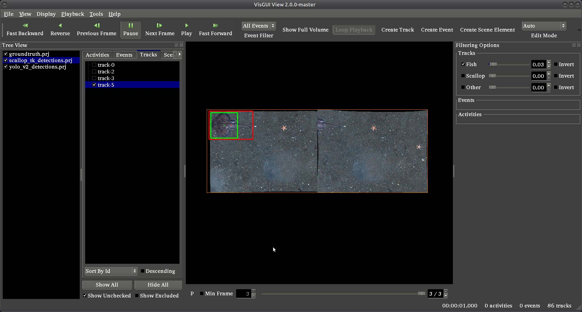
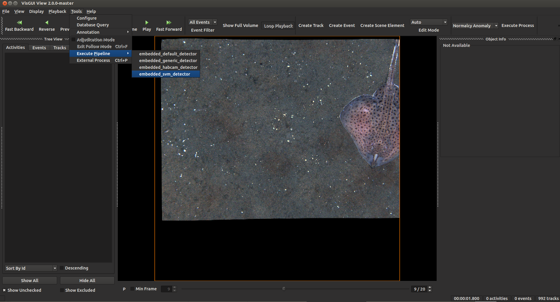
Running Examples in the GUI
The annotation GUI can also be used to run object detector or tracking pipelines. To accomplish this, load imagery using the annotation gui, then select Tools -> Execute Pipeline and select a pipeline to run, see below. Special notes: the ‘habcam’ pipeline only processes the left sides of images, assuming that the image contains side-by-side stereo pairs, and the ‘svm’ pipeline requires ‘.svm’ model files to exist in a ‘category_models’ directory from where the GUI is run. New pipelines can be added to the GUI by adding them to the default pipelines folder, with the word ‘embedded’ in them by default.
Build Requirements
These are the build flags required to run these examples, if building from the source. In the pre-built binaries they are all enabled by default.
Running Detectors From C++ Code
We will be using a Hough circle detector as an and example of the mechanics of implementing a VIAME detector in cxx code.
In general, detectors accept images and produce detections. The data types that we will need to get data in and out of the detector are implemented in the Vital portion of KWIVER. For this detector, we will be using an image_container to hold the input image and a detected_object_set to hold the detected objects. We will look at how these data types behave a little later.
Vital provides an algorithm to load an image. We will use this to get the images for the detector. The image_io algorithm provides a method that accepts a file name and returns an image.
kwiver::vital::image_container_sptr load(std::string const& filename) const;
Now that we have an image, we can pass it to the detector using the following method on hough_circle_detector and get a list of detections.
virtual vital::detected_object_set_sptr detect( vital::image_container_sptr image_data ) const;
The detections, for example, can be drawn on the original image to see how well the detector is performing.
The following program implements a simple single object detector.
#include <arrows/ocv/image_container.h>
#include <arrows/ocv/image_io.h>
#include <arrows/ocv/hough_circle_detector.h>

#include <string>

int main( int argc, char* argv[] )
{
  // get file name for input image
  std::string filename = argv[1];

  // create image reader
  kwiver::vital::algo::image_io_sptr image_reader( new kwiver::arrows::ocv::image_io() );

  // Read the image
  kwiver::vital::image_container_sptr the_image = image_reader->load( filename );

  // Create the detector
  kwiver::vital::algo::image_object_detector_sptr detector( new kwiver::arrows::ocv::hough_circle_detector() );

  // Send image to detector and get detections.
  kwiver::vital::detected_object_set_sptr detections = detector->detect( the_image );

  // See what was detected
  std::cout << "There were " << detections->size() << " detections in the image." << std::endl;

  return 0;
}
This sample program implements the essential steps of a detector.
Now that we have a simple program running, there are two concepts that are supported by vital that are essential for building larger applications; logging and configuration support.
Logging
Vital provides logging support through macros that are used in the code to format and display informational messages. The following piece of code implements a logger and generates a message.
// Include the logger interface
#include <vital/logger/logger.h>

// get a logger or logging object
kwiver::vital::logger_handle_t logger( kwiver::vital::get_logger( "test_logger" ));

float data;

// log a message
LOG_ERROR( logger, "Message " << data );
The vital logger is similar to most loggers in that it needs logging object to provide context for the log message. Each logger object has an associated name that can be used to when configuring what logging output should be displayed. The default logger does not provide any logger output control, but there are optional logging providers which do.
There are logging macros that produce a message with an associated severity, error, warning, info, debug, trace. The log text can be specified as an output stream expression allowing type specific output operators to provide formatting. The output line in the above example could have been written as a log message.
kwiver::vital::logger_handle_t logger( kwiver::vital::get_logger( "detector_test" ));
LOG_INFO( logger, "There were " << detections->size() << " detections in the image." );
Note that log messages do not need an end-of-line at the end.
Refer to the separate logger documentation for more details.
Detector Configuration Support
In our detector example we just used the detector in its default state without specifying any configuration options. This works well in this example, but there are cases and algorithms where the behaviour needs to be modified for best results.
Vital provides a configuration package that implements a key/value scheme for specifying configurable parameters. The config parameters are used to control an algorithm and in later examples it can be used to select the algorithm. The usual approach is to create a config structure from the contents of a file, but the values can be programatically set also. The key for a config entry has a hierarchical format
The full details of the config file structure are available in a separate document.
All algorithms support the methods get_confguration() and set_configuration(). The get_confguration() method returns a structure with the expected configuration items and default parameters. These parameters can be changed and sent back to the algorithm with the set_configuration() method. The hough_circle_detector, the configuration is as follows:
dp = 1

Description: Inverse ratio of the accumulator resolution to the
image resolution. For example, if dp=1 , the accumulator has the same
resolution as the input image. If dp=2 , the accumulator has half as
big width and height.

max_radius = 0

Description: Maximum circle radius.

min_dist = 100

Description: Minimum distance between the centers of the detected
circles. If the parameter is too small, multiple neighbor circles may
be falsely detected in addition to a true one. If it is too large,
some circles may be missed.

min_radius = 0

Description: Minimum circle radius.

param1 = 200

Description: First method-specific parameter. In case of
CV_HOUGH_GRADIENT , it is the higher threshold of the two passed to
the Canny() edge detector (the lower one is twice smaller).

param2 = 100

Description: Second method-specific parameter. In case of
CV_HOUGH_GRADIENT , it is the accumulator threshold for the circle
centers at the detection stage. The smaller it is, the more false
circles may be detected. Circles, corresponding to the larger
accumulator values, will be returned first.
Lets modify the preceding detector to accept a configuration file.
#include <vital/config/config_block_io.h>
#include <arrows/ocv/image_container.h>
#include <arrows/ocv/image_io.h>
#include <arrows/ocv/hough_circle_detector.h>

#include <string>

int main( int argc, char* argv[] )
{
  // (1) get file name for input image
  std::string filename = argv[1];

  // (2) Look for name of config file as second parameter
  kwiver::vital::config_block_sptr config;
  if ( argc > 2 )
  {
    config = kwiver::vital::read_config_file( argv[2] );
  }

  // (3) create image reader
  kwiver::vital::algo::image_io_sptr image_reader( new kwiver::arrows::ocv::image_io() );

  // (4) Read the image
  kwiver::vital::image_container_sptr the_image = image_reader->load( filename );

  // (5) Create the detector
  kwiver::vital::algo::image_object_detector_sptr detector( new kwiver::arrows::ocv::hough_circle_detector() );

  // (6) If there was a config structure, then pass it to the algorithm.
  if (config)
  {
    detector->set_configuration( config );
  }

  // (7) Send image to detector and get detections.
  kwiver::vital::detected_object_set_sptr detections = detector->detect( the_image );

  // (8) See what was detected
  std::cout << "There were " << detections->size() << " detections in the image." << std::endl;

  return 0;
}
We have added code to handle the optional second command line parameter in section (2). The read_config_file() function converts a file to a configuration structure. In section (6), if a config block has been created, it is passed to the algorithm.
The configuration file is as follows. Note that parameters that are not specified in the file retain their default values.
dp = 2
min_dist = 120
param1 = 100
Configurable Detector Type
To further expand on our example, the actual detector algorithm can be selected at run time based on the contents of our config file.
#include <vital/algorithm_plugin_manager.h>
#include <vital/config/config_block_io.h>
#include <vital/algo/image_object_detector.h>
#include <arrows/ocv/image_container.h>
#include <arrows/ocv/image_io.h>

#include <string>

int main( int argc, char* argv[] )
{
  // (1) Create logger to use for reporting errors and other diagnostics.
  kwiver::vital::logger_handle_t logger( kwiver::vital::get_logger( "detector_test" ));

  // (2) Initialize and load all discoverable plugins
  kwiver::vital::algorithm_plugin_manager::load_plugins_once();

  // (3) get file name for input image
  std::string filename = argv[1];

  // (4) Look for name of config file as second parameter
  kwiver::vital::config_block_sptr config = kwiver::vital::read_config_file( argv[2] );

  // (5) create image reader
  kwiver::vital::algo::image_io_sptr image_reader( new kwiver::arrows::ocv::image_io() );

  // (6) Read the image
  kwiver::vital::image_container_sptr the_image = image_reader->load( filename );

  // (7) Create the detector
  kwiver::vital::algo::image_object_detector_sptr detector;
  kwiver::vital::algo::image_object_detector::set_nested_algo_configuration( "detector", config, detector );

  if ( ! detector )
  {
    LOG_ERROR( logger, "Unable to create detector" );
    return 1;
  }

  // (8) Send image to detector and get detections.
  kwiver::vital::detected_object_set_sptr detections = detector->detect( the_image );

  // (9) See what was detected
  std::cout << "There were " << detections->size() << " detections in the image." << std::endl;

  return 0;
}
Since we are going to select the detector algorithm at run time, we no longer need to include the hough_circle_detector header file. New code in section (2) initializes the plugin manager which will be used to instantiate the selected algorithm at run time. The plugin architecture will be discussed in a following section.
The following config file will select and configure our favourite hough_circle_detector
# select detector type
detector:type =   hough_circle_detector

# specify configuration for selected detector
detector:hough_circle_detector:dp =           1
detector:hough_circle_detector:min_dist =     100
detector:hough_circle_detector:param1 =       200
detector:hough_circle_detector:param2 =       100
detector:hough_circle_detector:min_radius =   0
detector:hough_circle_detector:max_radius =   0
First you will notice that the config file entries have a longer key specification. The ‘:’ character separates the different levels or blocks in the config and enable scoping of the value specifications.
The “detector” string in the config file corresponds with the “detector” string in section (7) of the example. The “type” key for the “detector” algorithm specifies which detector is to be used. If an alternate detector type “foo” were to be specified, the config would be as follows.
# select detector type
detector:type =             foo
detector:foo:param1 =       20
detector:foo:param2 =       10
Since the individual detector (or algorithm) parameters are effectively in their own namespace, configurations for multiple algorithms can be in the same file, which is exactly how more complicated applications are configured.
Sequencing One or More Algorithms in a Pipeline
In a real application, the input images may come from places other than a file on the disk and there may be algorithms applied to precondition the images prior to object detection. After detection, the detections could be overlaid on the input imagery or compared against manual annotations.
Ideally this type of application could be structured to flow the data from one algorithm to the next, but writing this a one monolithic application, changes become difficult and time consuming. This is where another component of KWIVER, sprokit, can be used to simplify creating a larger application from smaller component algorithms.
Sprokit is the “Stream Processing Toolkit”, a library aiming to make processing a stream of data with various algorithms easy. It provides a data flow model of application building by providing a process and interconnect approach. An application made from several processes can be easily specified in a pipeline configuration file.
Lets first look at an example application/pipeline that runs our hough_circle_detector on a set of images, draws the detections on the image and then displays the annotated image.
# ================================================================
process input
  :: frame_list_input
  :image_list_file    images/image_list_1.txt
  :frame_time          .3333
  :image_reader:type   ocv

# ================================================================
process detector
  :: image_object_detector
  :detector:type    hough_circle_detector
  :detector:hough_circle_detector:dp            1
  :detector:hough_circle_detector:min_dist      100
  :detector:hough_circle_detector:param1        200
  :detector:hough_circle_detector:param2        100
  :detector:hough_circle_detector:min_radius    0
  :detector:hough_circle_detector:max_radius    0

# ================================================================
process draw
  :: draw_detected_object_boxes
  :default_line_thickness 3

# ================================================================
process disp
  :: image_viewer
  :annotate_image         true
  # pause_time in seconds. 0 means wait for keystroke.
  :pause_time             1.0
  :title                  NOAA images

# ================================================================
# connections
connect from input.image
        to   detector.image

connect from detector.detected_object_set
        to   draw.detected_object_set
connect from input.image
        to draw.image

connect from input.timestamp
        to   disp.timestamp
connect from draw.image
        to   disp.image

# -- end of file --
Our example pipeline configuration file is made up of process definitions and connections. The first process handles image input and uses a configuration style we saw in the description of selectable algorithms, to select an “ocv” reader algorithm. The next process is the detector, followed by the process that composites the detections and the image. The last process displays the annotated image. The connections section specify how the inputs and outputs of these processes are connected.
This pipeline can then be run using the ‘kwiver runner ‘ app